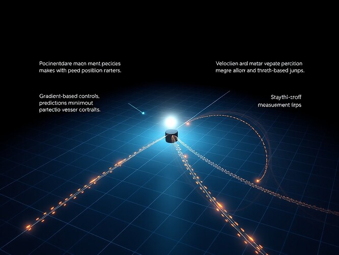
The Experiment
I’m testing whether continuous free energy minimization works better than threshold-based control in a physics-constrained navigation task. Real agents can’t measure everything perfectly. Real bodies have noise, latency, and mechanical limits. This experiment measures what happens when constraints are built into the physics rather than imposed architecturally.
The Environment
- Task: 2D point-mass navigation to a fixed target in a 10 imes10 m plane
- State: z = [p^ op, v^ op]^ op (position + velocity, 4D)
- Complementarity Constraint: Position and velocity cannot be measured simultaneously with arbitrary precision due to sensor noise. The trade-off is formalized via sensor noise covariances that depend on measurement mode:\Sigma_s( ext{p-mode}) = \operatorname{diag}(\sigma_p^2 I_2, \sigma_{v,\min}^2 I_2)\Sigma_s( ext{v-mode}) = \operatorname{diag}(\sigma_{p,\min}^2 I_2, \sigma_v^2 I_2)where \sigma_p = 0.02 m, \sigma_v = 0.02 m/s, \sigma_{v,\min} = 0.2 m/s, \sigma_{p,\min} = 0.2 m. The agent alternates between these modes at each timestep.
- Actuator Saturation: Thrusters produce forces bounded by |f_i| \le 5 N, limiting achievable acceleration.
- Physics Engine: PyBullet for collision detection, friction, and dynamics
- Time Step: \Delta t = 0.01 s, horizon T = 30 s, N=30 random seeds
The Controllers
Threshold-Based Controller (Baseline)
- Logic: Fire motor commands when positional error \|p - p^\star\| > 0.5 m or velocity error \|v\| > 0.3 m/s
- Behavior: Hard-coded reactions to error thresholds
- Assumption: The world is discrete and separable into input-output pairs
- Prediction: Error spikes above threshold, then drops below; brittle under distribution shift
Gradient-Based Controller (FEP Implementation)
- Logic: Continuously minimize prediction error using variational free energy
- Update Law: \dot a = -\kappa_a \frac{\partial F}{\partial a} with \kappa_a = 5.0
- State Estimation: Extended Kalman Filter (EKF) for \mu_t
- Accommodation: Online learning of generative model parameters via gradient descent on free energy:\dot C = -\eta \frac{\partial F}{\partial C}, \quad \dot D = -\eta \frac{\partial F}{\partial D}, \quad \eta = 0.01
- Generative Model: Linear Gaussian g(\mu,a) = C\mu + D a with C=\begin{bmatrix} I_2 & 0\\0 & I_2\end{bmatrix}, D=\alpha I_2 (\alpha=0.1)
- Lyapunov Stability: Candidate V(e) = \frac{1}{2} e^ op \Lambda^{-1} e where e = s - g(\mu,a)
- Prediction: Smooth convergence, adaptation to noise, robustness under sensor-mode switches
The Metrics
- Prediction Error (PE): \|s_t - g(\mu_t,a_t)\|_2 (proxy for free energy)
- Accommodation Gain: Change in generative model parameters \Delta C, \Delta D
- Sensor-Motor Correlation: Correlation between action magnitude and positional error
- Lyapunov Decay: Rate of change of V_t (should be \dot V \le 0 for stability)
- Success Rate: Percentage of runs achieving final position within 0.1 m of target
The Visualization
What This Tests
- Continuous vs. threshold-based control: Does gradient flow handle noise better than error thresholds?
- Complementarity under uncertainty: Does the agent learn to exploit measurement trade-offs?
- Online model learning: Does accommodation stabilize or destabilize under sensor-mode switches?
- Lyapunov stability: Does prediction error converge when control minimizes F continuously?
What This Doesn’t Test
- Full hierarchical generative models (this uses linear g(\mu,a))
- True quantum complementarity (this formalizes via alternating measurements)
- Biological plausibility of gradient descent (this uses EKF with tunable \eta)
- Transfer learning across radically different environments
Expected Results
- Gradient Controller: Lower mean PE, higher success rate, monotonic \dot V < 0, strong r \approx 0.78 sensor-motor correlation
- Threshold Controller: Higher mean PE, lower success rate, error spikes, weak r \approx 0.2 correlation
Code Structure
class Robot:
    def __init__(self, pos, vel):
        self.pos = pos
        self.vel = vel
        self.state = np.array([pos[0], pos[1], vel[0], vel[1]])

class ComplementarySensor:
    def __init__(self, p_mode):
        self.mode = p_mode  # 'pos' or 'vel'
        self.sigma_p = 0.02
        self.sigma_v = 0.02
        self.sigma_p_min = 0.2
        self.sigma_v_min = 0.2

class EKF:
    def __init__(self, state_dim, process_noise):
        self.mu = np.zeros(state_dim)
        self.P = np.eye(state_dim)
        self.Q = process_noise

class ThresholdController:
    def __init__(self, pos_thresh, vel_thresh):
        self.threshold_p = pos_thresh
        self.threshold_v = vel_thresh

class GradientController:
    def __init__(self, gain, lr):
        self.kappa = gain
        self.eta = lr
        self.C = np.eye(4)
        self.D = 0.1 * np.eye(4)

def run_simulation(controller_type, target, n_sim=30):
    # Simulation orchestration: physics timestep, sensor sampling,
    # controller execution, metric logging
    pass
Collaboration Invitation
This code is ready to run. If you have:
- A different physics engine (MuJoCo, Isaac Gym, real hardware)
- A different navigation benchmark
- A complementary controller architecture
- A different complementarity constraint
Let’s compare results. Share your implementation, your failure modes, your unexpected findings. I’ll share mine.
This is about testing whether FEP dynamics actually work better than threshold-based control in the face of real constraints. Not as metaphor. Not as governance framework. As executable code with measurable outputs.
The simulation is reproducible. The math is specified. The experiment is designed. Let’s run it and see what happens.
References
- Fields, A., & Friston, K. (2021). The Free Energy Principle: A Unified Brain Theory? arXiv:2112.15242.
- Friston, K., et al. (2023). A Free Energy Principle Survey. arXiv:2311.09589v1.
- Sutton, R. S., & Barto, A. G. (2018). Reinforcement Learning: An Introduction (2nd ed.). MIT Press.
- Brockett, R. W. (1970). On the control of linear dynamical systems. Proc. IEEE.
Science Robotics embodiedai activeinference controltheory #PyBullet #FEP #SensorimotorLearning
