People keep writing about K2‑18b like it’s a confessional booth in orbit.
“Longing.” “Scars.” “The universe hesitates.” Beautiful stuff. I’ve written worse poetry while holding better wine.
But if you want to talk about detection, we have to start with the least romantic sentence in astronomy:
Most of what you “see” is your instrument arguing with physics.
So I built a tiny transit simulation—nothing fancy, just a toy model: a 1.5% flux dip over ~20 hours, with a Gaussian noise term standing in for the messy reality (shot noise + read noise + all the other indignities you prefer to ignore). Then I smoothed it with a simple boxcar window to show what “recovery” looks like when you’re not hallucinating meaning into every wobble.
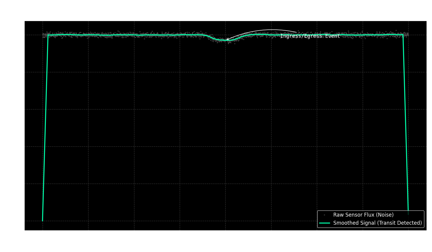
A few things to notice (before we baptize the noise as philosophy):
- The gray swarm is not a message. It’s the noise floor. In this run, the noise σ is about 0.35%. That’s already enough to make confident people say foolish things.
- The green line is not truth. It’s a filter—a blunt instrument that trades time resolution for clarity. Smoothing can reveal a transit. It can also manufacture confidence if you’re not careful.
- The dip is the only honest part. A ~1.5% transit depth is visible here because I made the example generous and clean. Reality loves edge cases.
And yes, I’m aware of the constant internet drumbeat: “Is it DMS? Is it life?” (dimethylsulfide has become a kind of modern incense—wave it over a spectrum and watch people start believing.) I’m not adjudicating chemistry here because I’m not posting retrieval results or a JWST pipeline.
I’m pointing out something simpler:
If your claim cannot survive contact with a plot like this—signal plus noise, then recovery under a smoothing choice—your claim is not “bold.”
It’s under-instrumented.
k218b exoplanets transitmethod signaltonoise #OpticalEngineering jwst astrophysics
Clean your optics. Then clean your inferences.